Google Sheets Budget Template: Free Download and Setup Guide
A complete guide to setting up a powerful budget tracking spreadsheet in Google Sheets, with automated calculations, visual charts, and a monthly review workflow.
Every budgeting app I’ve tried has one fatal limitation: it thinks it knows better than I do how to categorize my spending. Google Sheets doesn’t think anything — it does exactly what you tell it to. After helping friends and family set up their first budget spreadsheets, I’ve refined a template that balances simplicity with insight. No VBA macros, no complex scripting — just clean formulas that a spreadsheet beginner can understand and customize.
Why Google Sheets Beats Most Budgeting Apps
Before building, let’s understand why a spreadsheet is genuinely powerful for personal finance:
Unlimited customization: Your spending categories are unique. A freelance graphic designer’s budget looks nothing like a salaried IT professional’s. Apps impose their categories; Sheets lets you create yours.
Full data ownership: Your financial data stays in your Google account. No third-party company mines it for insights or sells anonymized patterns to advertisers.
Zero cost: Every feature of Google Sheets is free. No “upgrade to Premium for charts” or “Pro required for bank sync.”
Cross-device access: Works on any browser, any phone, any tablet. Real-time sync means your budget is always current.
Longevity: Apps get discontinued, change pricing, or remove features. Google Sheets has been stable for 15+ years. Your budget data from 2024 will still be accessible in 2034.
The Template Structure
Our budget template has four sheets (tabs):
Sheet 1: Monthly Budget
This is your main working sheet. Structure:
Row 1: Month selector (dropdown: January through December) Row 2-3: Headers
Columns:
- A: Category name
- B: Budgeted amount (your planned spending)
- C: Actual amount (what you really spent)
- D: Difference (auto-calculated: B minus C)
- E: Status (conditional formatting: green if under, red if over)
Rows organized by section:
- Income section (salary, freelance, interest)
- Fixed expenses (rent, EMIs, insurance)
- Variable expenses (groceries, transport, utilities)
- Discretionary (dining, entertainment, shopping)
- Savings & investments (SIPs, emergency fund, goals)
Key formulas:
- Total Income:
=SUM(C3:C5)(adjust range for your income rows) - Total Expenses:
=SUM(C7:C25)(adjust for expense rows) - Savings Rate:
=(Total Income - Total Expenses) / Total Income * 100 - Category Difference:
=B7-C7(positive means under budget)
Sheet 2: Transaction Log
A raw data entry sheet where you log individual transactions:
| Date | Amount | Category | Payment Method | Note |
|---|---|---|---|---|
| 01-Apr | 250 | Groceries | UPI | Vegetables |
| 01-Apr | 150 | Transport | Cash | Auto to office |
| 02-Apr | 499 | Subscription | Card | Spotify annual |
This feeds into Sheet 1 via SUMIFS formulas that automatically total transactions by category for the selected month.
Key formula: =SUMIFS('Transaction Log'!B:B, 'Transaction Log'!C:C, A7, MONTH('Transaction Log'!A:A), selected_month)
This formula says: “Sum all amounts from the Transaction Log where the Category matches this row’s category AND the month matches the selected month.”
Sheet 3: Annual Overview
A 12-column summary showing each month’s total spending by category. Auto-populated from the Transaction Log using the same SUMIFS approach.
This sheet reveals spending trends that are invisible in monthly views. You might not notice that your dining spending increased by ₹500 per month — but the annual view shows a clear upward slope from ₹3,000 in January to ₹6,000 in June.
Embedded chart: A stacked bar chart showing spending by category across months. This single visualization is the most valuable financial insight tool in the entire template.
Sheet 4: Settings & Reference
- Category list (used for data validation dropdowns)
- Payment method list
- Your income details
- Financial goals with progress tracking
Building It Step by Step
Step 1: Create the Category Structure (10 minutes)
Open a new Google Sheet and create your categories. Be specific but not granular — you want 12-18 categories, not 40. Here’s a proven starting list:
Income: Salary, Freelance, Interest/Dividends, Other Fixed: Rent, Loan EMI, Insurance, Subscriptions Variable: Groceries, Electricity, Water, Internet/Phone, Transport Discretionary: Dining Out, Entertainment, Clothing, Personal Care, Gifts/Social Savings: Emergency Fund, Mutual Funds/SIP, Goal Savings
Step 2: Add the Formulas (15 minutes)
For each category row:
- Column D (Difference):
=B[row]-C[row] - Column E (Status):
=IF(D[row]>=0, "✅ Under", "🔴 Over")
For summary rows:
- Total Income:
=SUM(income_range) - Total Expenses:
=SUM(expense_range) - Net Savings:
=Total_Income - Total_Expenses - Savings Rate:
=Net_Savings / Total_Income
Step 3: Apply Conditional Formatting (5 minutes)
Select the Difference column. Add conditional formatting:
- Values ≥ 0: Green background
- Values < 0: Red background
This creates instant visual feedback — you can scan the entire budget in seconds and see which categories are healthy (green) and which need attention (red).
Step 4: Set Up Data Validation (5 minutes)
In the Transaction Log, add dropdown validation for:
- Category column: pulls from your Settings sheet category list
- Payment Method: pulls from your payment methods list
This prevents typos that would break your SUMIFS formulas and ensures consistency.
Step 5: Create Charts (10 minutes)
Insert two charts:
- Pie chart: Monthly spending by category (from Monthly Budget sheet)
- Bar chart: Monthly spending trend (from Annual Overview sheet)
Anchor the pie chart in the Monthly Budget sheet for quick visual reference.
Weekly and Monthly Workflow
During the week: Log transactions in the Transaction Log. Total time: 3-5 minutes per week (or use the Saturday batch entry method).
Month-end review (10 minutes):
- Verify all transactions are logged
- Check the Monthly Budget sheet — formulas auto-calculate everything
- Review which categories went over/under
- Adjust next month’s budget amounts based on insights
- Glance at the Annual Overview for trends
Pro Tips
Freeze header rows: Select Row 2, go to View → Freeze → Up to rows. This keeps your headers visible while scrolling through transactions.
Use named ranges: Instead of SUM(C7:C25), create a named range called “AllExpenses” for cleaner, more readable formulas.
Mobile-friendly entry: Pin the Google Sheets shortcut to your home screen. The mobile app’s entry experience is clean enough for quick transaction logging.
Backup monthly: At the end of each month, use File → Make a Copy to save a backup. This protects against accidental formula deletion and gives you a clean archive.
The Most Important Thing
The template doesn’t need to be perfect. Starting with a basic version and improving it monthly is far more effective than spending hours building an elaborate system you never use. Begin with just the Transaction Log and Monthly Budget sheets. Add the Annual Overview after your first complete month of data. You’ll have a personalized, powerful financial tool that grows with your needs.
PayWise Team
Personal finance enthusiast and tech writer at PayWise. Passionate about making digital finance accessible to everyone through practical, experience-based guides.